This post is part of a series exploring in depth how large language models work. You can find the whole series here.
The remarkable capabilities of Large Language Models (LLMs) come with significant computational challenges, especially concerning GPU memory usage. One source of these challenges lies in what’s referred to as the Key-Value (KV) cache, a critical optimization technique employed in LLMs to ensure efficient token-by-token generation. This cache consumes significant amount of GPU memory to the point that it itself can limit LLM performance and context size.
This post covers KV cache optimization techniques. It starts with an explanation of how a basic KV cache works and then delves into various methods implemented by open-source models and frameworks to enhance its scalability and reduce its memory footprint.
I will assume a basic understanding of transformers and self-attention, though the most crucial concepts will be reviewed. The Illustrated Transformer is also a good source for beginners.
Table of contents
Open Table of contents
Motivation for the KV cache
During inference, an LLM generates its output token-by-token, a process known as autoregressive decoding. Each token generated depends on all previous tokens, including the tokens in the prompt and all previously generated output tokens. When this list of tokens grows large due to a lengthy prompt or a long output, the computations in the self-attention stage can become a bottleneck.
The KV cache resolves this bottleneck, maintaining a small and consistent performance for each decoding step, regardless of the token count.
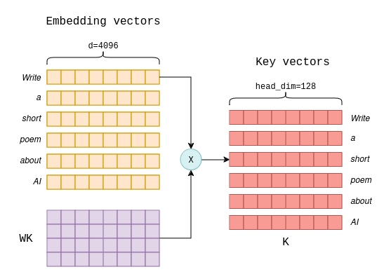
To see why it’s needed, recall that in a standard self-attention mechanism as originally proposed and used in models such as Llama-7B, three vectors are computed for each token, known as key, query and value vectors. These vectors are calculated using a simple matrix multiplication between the token’s embedding and the WK, WQ and WV matrices, which are part of the model’s learned parameters. Below is an illustration of the calculation of the key vectors of a prompt consisting of six tokens:
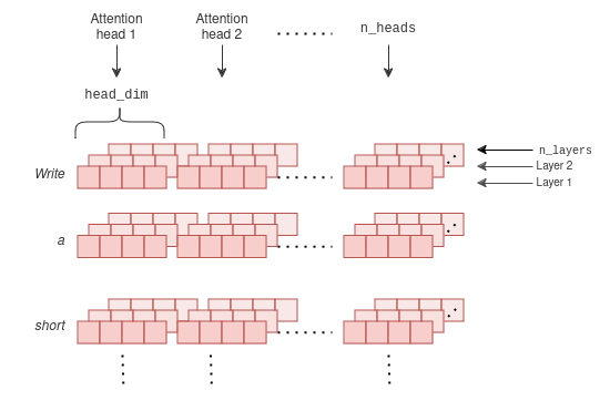
In a standard self-attention mechanism, there exist multiple parallel “heads” that perform self-attention independently.
Hence, the aforementioned process is repeated for each attention head and for each layer, each with different parameter matrices.
For instance, in Llama-7B, this would mean n_heads=32 and n_layers=32 just to generate a single token.
As the number of tokens increases, this matrix multiplication operation involves larger matrices and can saturate the GPU’s capacity. In an article called Transformer Inference Arithmetic, it is estimated that for a 52B parameter model running on an A100 GPU, performance begins to degrade at 208 tokens due to excessive floating-point operations performed in this stage.
The KV cache addresses this issue. The core idea is simple: during the successive generation of tokens, the key and value vectors computed for previous tokens remain constant. Instead of recalculating them each iteration and for each token, we can compute them once and cache them for future iterations.
A basic KV cache
The cache works as follows:
- In the initial decoding iteration, the key and value vectors are computed for all the input tokens, as shown in the above diagram. These vectors are then stored in a tensor in the GPU’s memory, serving as a cache. When the iteration ends, a new token is generated.
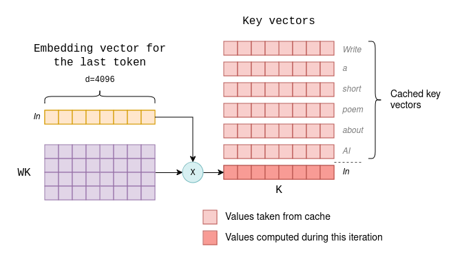
- In subsequent decoding iterations, only the key and value vectors for the newly generated token are calculated.
The cached key and value vectors from previous iterations, along with the ones for the new token, are concatenated to form the
KandVmatrices required for self-attention. This eliminates the need to recalculate the key and value vectors for all previous tokens. The new key and value vectors are also appended to the cache.
For instance, suppose the first iteration generates the token “In” (that’s what ChatGPT likes to start its poems with). The second iteration would then proceed as follows (compare with the previous diagram):
As a result, the computational overhead of each successive generation remains small and consistent. That is why LLMs have distinct performance metrics for the first token and for subsequent tokens, referred to as Time to First Token and Time Per Output Token, respectively. To generate the first token, all key and value vectors must be computed, whereas for subsequent tokens, only one key and one value vectors are computed.
You might wonder why we don’t cache the query vectors as well. The answer is that, having cached the key and value vectors, the query vectors for previous tokens become unnecessary in subsequent iterations. Only the query vector of the latest token is needed to compute self-attention. I explained this bit more in depth in a previous blog post.
The size of the cache
Just how large the KV cache has to be? For every token, it needs to store two vectors for each attention head and for each layer. Each element in the vector is a 16-bit floating-point number. So for each token, the memory in bytes in the cache is:
2 * 2 * head_dim * n_heads * n_layersWhere head_dim is the size of the key and value vectors, n_heads the number of attention heads and n_layers the number of layers in the model.
Substituting the parameters of Llama 2:
| Model | Cache size per token |
|---|---|
| Llama-2-7B | 512KB |
| Llama-2-13B | 800KB |
If you are familiar with Numbers every LLM Developer should know, they claim each output token requires approximately 1MB of GPU memory. That’s where this number comes from.
Now, this calculation is for each token. To accommodate the full context size for a single inference task, we must allocate enough cache space accordingly. Moreover, if we run inference in batches (i.e. on multiple prompts simultaneously once), the cache size is multiplied again. Therefore, the full size of the cache is:
2 * 2 * head_dim * n_heads * n_layers * max_context_length * batch_sizeIf we want to utilize the entire Llama-2-13B context of 4096 tokens, in batches of 8, the size of the cache would be 25GB, almost as much as the 26GB needed to store the model parameters. That’s tons of GPU memory!
So the size of the KV cache limits two things:
- The maximum context size that can be supported.
- The maximum size of each inference batch.
The rest of this post delves into commonly employed techniques to reduce the cache size.
Grouped-query Attention
Grouped-query attention (GQA) is a variation of the original multi-head attention that reduces the KV cache size while retaining much of the original performance. It is used in Llama-2-70B. To quote from the Llama-2 paper:
A standard practice for autoregressive decoding is to cache the key (K) and value (V) pairs for the previous tokens in the sequence, speeding up attention computation. With increasing context windows or batch sizes, however, the memory costs associated with the KV cache size in multi-head attention (MHA) models grow significantly. For larger models, where KV cache size becomes a bottleneck, key and value projections can be shared across multiple heads without much degradation of performance (Chowdhery et al., 2022). Either the original multi-query format with a single KV projection (MQA, Shazeer, 2019) or a grouped-query attention variant with 8 KV projections (GQA, Ainslie et al., 2023) can be used.
A model using GQA uses a reduced number of attention heads for key and value vectors, denoted n_kv_heads.
For the query vectors, the original number of attention heads n_heads is maintained.
The key and value vector pairs are then shared across multiple query heads.
This approach effectively reduces the KV cache size by a factor of n_heads / n_kv_heads.
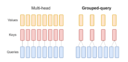
In Llama-2-70B, for example, n_heads = 64 and n_kv_heads = 8, reducing the cache size by a factor of 8.
Open-source models using GQA are summarized in the following table.
| Model | Cache size per token without GQA (hypothetical) | GQA factor | Cache size per token with GQA |
|---|---|---|---|
| Gemma-2B | 144KB | 8 | 18KB |
| Mistral-7B | 512KB | 4 | 128KB |
| Mixtral 8x7B | 1MB | 4 | 256KB |
| Llama-2-70B | 2.5MB | 8 | 320KB |
Sliding Window Attention
Sliding window attention (SWA) is a technique utilized by Mistral-7B to support longer context sizes without increasing the KV cache size.
SWA is a modification to the original self-attention mechanism.
In the original self-attention, a score is computed for each token with all its preceding tokens, using their key and query vectors.
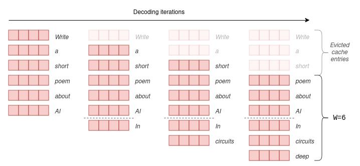
In SWA on the other hand, a fixed window size W is selected, and the scores are calculated between each token and its preceding W tokens only.
Essentially, this implies that only the latest W key and value vectors need to be retained in the cache.
As decoding progresses and the number of tokens exceeds W, older key and value vectors are evicted from the cache using a sliding window, as they are no longer necessary.
The trick here is that model can still attend to tokens older than W due to the layered architecture of the transformer.
Information regarding older tokens is stored in the key and value vectors of the upper layers of the transformer.
Theoretically, the model can attend to W * n_layers tokens while only keeping W vectors in the cache, though with diminishing abilities.
A more detailed explanation can be found in the Mistral paper.
In practice, Mistral-7B uses W=4096, with an officially supported context size of context_len=8192.
SWA therefore reduces the KV cache size up to a factor of 2, in addition to the factor of 4 from GQA.
PagedAttention
PagedAttention is a sophisticated cache management layer popularized and used by the vLLM inference framework.
The motivation behind PagedAttention is identical to GQA and SWA: it aims to reduce the KV cache size to enable longer context lengths and larger batch sizes. In high-scale inference scenarios, processing large batches of prompts can result in increased throughput of output tokens.
However, PagedAttention does not alter the model’s architecture; instead, it operates as a cache management layer that seamlessly integrates with any of the previously mentioned attention mechanisms (multi-head, GQA, and SWA). Consequently, it can be utilized with all modern open-source LLM models.
PagedAttention makes two key observations:
- There exists significant memory wastage in the KV cache due to over-reservation: The maximum memory required to support the full context size is always allocated, but seldom fully utilized.
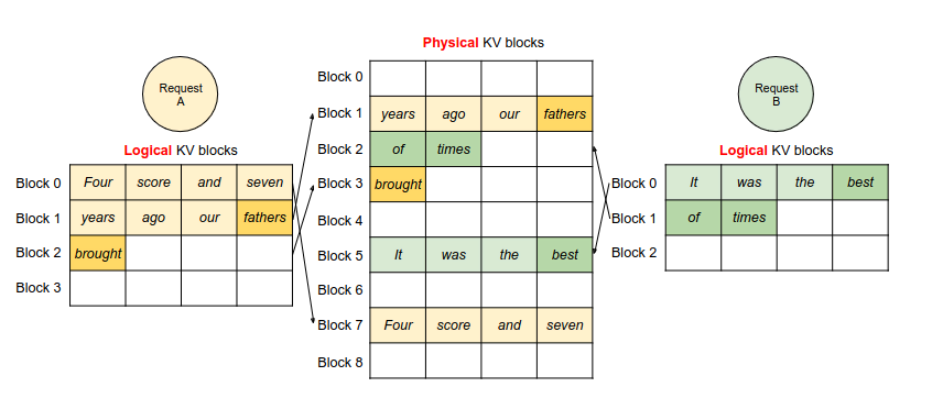
- In scenarios where multiple inference requests share the same prompt, or at least its beginning, the key and value vectors for the initial tokens are identical and could be shared among requests. This scenario is particularly common in applicative requests that share a large initial system prompt.
PagedAttention manages the cache entries similarly to how an operating system manages virtual and physical memory:
- Physical GPU memory is not pre-allocated.
- When new cache entries are saved, PagedAttention allocates new physical GPU memory in non-contiguous blocks.
- A dynamic mapping table maps between the virtual view of the cache as a contiguous tensor and the non-continguous physical blocks.
This solves the over-reservation issue, reducing memory wastage from 60-80% to 4% according to their research. Moreover, the mapping table lets multiple inference requests reuse the same cache entries if they share the same initial prompt.
If you want to learn more, the vLLM site and paper contain very easy-to-digest visualizations of this mechanism at work.
Distributed KV cache across multiple GPUs
Closed-source models have all recently increased their supported context size significantly. GPT-4, for instance, now accommodates a context of 128k tokens, while Gemini 1.5 claims to support up to 1M tokens. However, when utilizing these huge contexts, the KV cache may exceed the available memory on a single GPU.
For example, assuming GPT-4’s per-token memory is 1MB (a pure guess), utilizing the full context would necessitate approximately 128GB of GPU memory, exceeding the capacity of a single A100 card.
Distributed inference involves running LLM requests across multiple GPUs. While this offers additional advantages, it also enables the KV cache to exceed the memory of a single GPU.
The way it works is, at least theoretically, rather simple: Since the self-attention mechanism is composed of multiple heads working independently, it can be distributed across multiple GPUs. Each GPU is assigned a subset of attention heads to execute. The key and value vectors for each attention head are then cached in the memory of the allocated GPU. When finished, the results of all attention heads are collected to a single GPU where they are combined for use in the rest of the transformer layer. This approach allows for distributing the cache across as many GPUs as there are attention heads, for instance, up to 8 for Llama-70b.
Frameworks like vLLM offer distributed inference capabilities out of the box.
Summary
To summarize:
- The KV cache is a crucial optimization technique employed in LLMs to maintain a consistent and efficient per-token generation time.
- However, it comes with a significant cost to GPU memory, potentially requiring multiple MB per token.
- To reduce this memory footprint, open-source models leverage modified attention mechanisms called Grouped-query attention (GQA) and Sliding window attention (SWA).
- PagedAttention, implemented in the vLLM framework, is a transparent cache management layer that reduces memory wastage in GPUs incurred by the KV cache.
- To support huge contexts with hundreds of thousands of tokens, models may distribute their KV cache across multiple GPUs.
It would definitely be interesting to watch for developments in this area as open-source models catch up with their closed-source counterparts in terms of huge context sizes, which would necessitate further optimizations.